Use Python 373 Write Function Ticker First Runs Reads Txt File Stores Returned Dictionary Q43800969

Use python 3.7.3

Write a function ticker() that first runs readsa txt file, and then stores the returned dictionary. It then runsan interactive loop with the user in which the user is prompted fora company name. If the company name (key) is in the dictionary,then its ticker form and the IPO year is printed. Otherwise awarning is printed that the company name is not in the list. If theuser just hits return without entering a name, the loop stops.

>>> ticker()

Company name: Amazon.com

No ticker symbol on record for Amazon.com

Company name: Americao

No ticker symbol on record for Americao

Company name: Morningstar, Inc.

Morningstar, Inc. has ticker MORN. IPO: 2005

Company name:

>>>

nasdaq.txt :
TFSC   1347 Capital Corp.   2014
TFSCR   1347 Capital Corp.   2014
TFSCU   1347 Capital Corp.   2014
TFSCW   1347 Capital Corp.   2014
PIH   “1347 Property Insurance Holdings,Inc.”   2014
FLWS   “1-800 FLOWERS.COM, Inc.”   1999
FCTY   “1st Century Bancshares, Inc”  n/a
FCCY   1st Constitution Bancorp (NJ)  n/a
SRCE   1st Source Corporation   n/a
VNET   “21Vianet Group, Inc.”   2011
TWOU   “2U, Inc.”   2014
DGLD   3X Inverse Gold ETN Velocityshares  n/a
DSLV   3X Inverse Silver ETN Velocityshares  n/a
UGLD   3X Long Gold ETN Velocityshares  n/a
USLV   3X Long Silver ETN Velocityshares  n/a
JOBS   “51job, Inc.”   2004
SIXD   “6D Global Technologies, Inc.”  n/a
CAFD   8point3 Energy Partners LP   2015
EGHT   8×8 Inc   n/a
AVHI   “A V Homes, Inc.”   n/a
SHLM   “A. Schulman, Inc.”   1972
AAON   “AAON, Inc.”   n/a
ABAX   “ABAXIS, Inc.”   1992
ABY   Abengoa Yield plc   2014
ABGB   “Abengoa, S.A.”   2013
ABEO   Abeona Therapeutics Inc.   n/a
ABEOW   Abeona Therapeutics Inc.   n/a
ABMD   “ABIOMED, Inc.”   n/a
AXAS   Abraxas Petroleum Corporation  n/a
ACTG   Acacia Research Corporation   n/a
ACHC   “Acadia Healthcare Company, Inc.”  n/a
ACAD   ACADIA Pharmaceuticals Inc.   1985

Expert Answer

Answer to Use python 3.7.3 Write a function ticker() that first runs reads a txt file, and then stores the returned dictionary. It…

Use Python Collage Football Event Photo Background Along Jackrabbit Antelope Photos Foregr Q43893691

1. use Python to collage a football event photo (background),along with a jackrabbit and antelope photos (foreground).
2. Trade the antelope horns with the jackrabbit ears to create 2possible candidates for a Jackalope.
3. Save the resulting (completed) image file.
4. Create an HTML Web document that displays the collaged imagefrom step 3. Add a headline “Mythological JackalopeDiscovered!”

Expert Answer

Answer to use Python to collage a football event photo (background), along with a jackrabbit and antelope photos (foreground). Tr…

Use Python Compute Step1 4 Already Compute Step1 3 Correct Code Step 1 3 Shown Picture Nee Q43818986

Use python to compute step1-4 (I already compute step1-3 and itis correct, the code of step 1-3 are shown at the picture below,only need help in step 4)PLEASE HELP ME!!! U need to numpy packagei imported?How can i send u the file?where can i find the numpycode?

• Step 1: Build a 2D square box (edge length = 2nm) containing a random arrangement of particles, each separated bya minimum distance of 0.24 nm.

• Step 2: Calculate the g(r) of theconfiguration built in Step 1, without normalising it withrespect to the ideal gas.

• Step 3: Build a number of configurations (suchas the one built in Step 1) sufficient to converge the g(r) of thesystem to an acceptable degree of accuracy. Compute the g(r) of thesystem and comment on why do you think you have generated enoughconfigurations.
• Step 4: Find the largest portion of emptyspace (i.e. void) within each of the configurations you havegenerated in Step 3. Calculate and visualize the probabilitydensity function of the largest void in the system as a function ofits size.

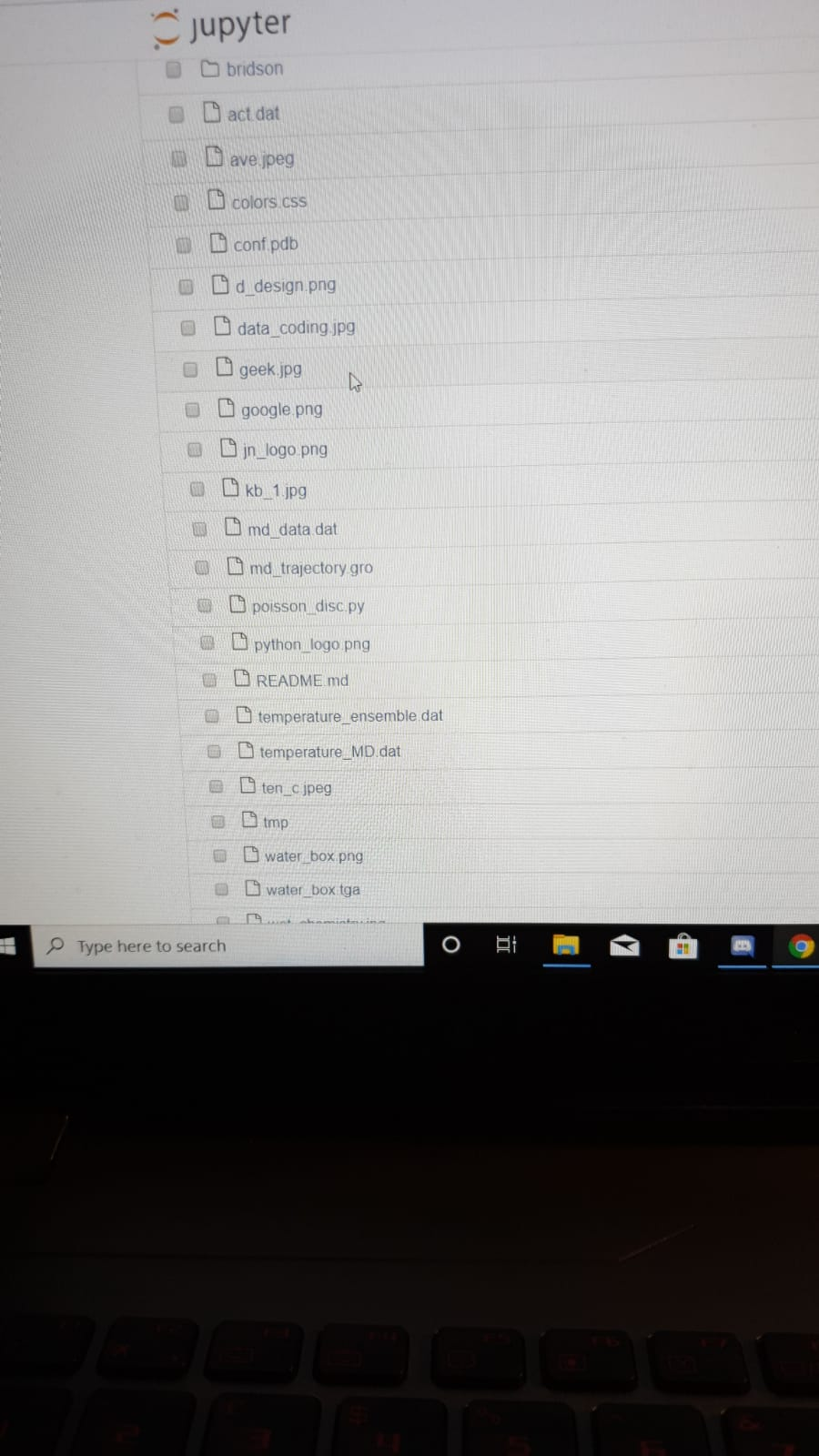
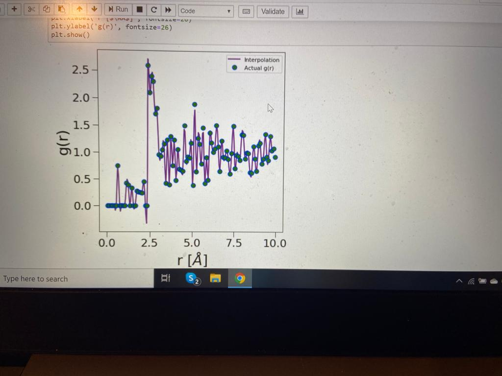
o jupyter bridson Dact dat Dave jpeg 0 colors css D confpdb d _design.png data_coding.jpg geek.jpg google png Din_logo.png 0 kb_1.jpg Omd_data dat O m d_trajectory gro poisson disc.py python_logo png D README.md temperature_ensemble dat temperature_MD.dat ten_c jpeg Dtmp water_box png water_box tga Type here to search Edit View Insert Help + Cell Kernel N Run O C Widgets Code Validate L. In [34]: # Import a number is useful packages… import numpy as np import matplotlib.pyplot as plt from scipy.interpolate import interpid from scipy.signal import argrelextrema from mpl_toolkits.mplot 3d import Axes 3D from STUFF.poisson_disc import Grid import random In [35]: #step 1 # Set the Length and width (the x and y dimensions) of the box length = 20.0 # can be any units you like. A meaningful choice: [A] width = length # This is a square 2D box # Set the minimum distance between the particles (as you can see, this is not really a hard sphere Liquid! why?) min_r = 2.4 # [A]rad_py # Generate a random arrangement of particles – according to an algorithm called Poisson sampling. # Note that every time you run this cell, the algorithm will generate a DIFFERENT configuration! grid = Grid(min_r, length, width) # Random seed rand = (random.uniform(e, length), random.uniform(e, width)) # Do the sampling data = grid.poisson(rand) In [36]: # We use “def” to tell Python we are defining a function here to search Edit View Insert Cell Kemel Widgets Help Trusted 8 B Run I C Code Validate w OLO POLODUIT anu) In [36]: # We use “def” to tell Python we are defining a function # “unzip” is the name of the function – I chose that. You can be creative, but long names are cumbersome to be called # Later on within the Notebook, and if the name of a function is the same as the name of a variable, things get ugly. def unzip(items): # The list of arguments given as input is passed in the brackets. In this case,”items # is the one and only argument required as input # We use “return” to tell Python this is the quantity we want to get as output anytime we call this function return ([item[i] for item in items] for i in range(Ten(items[0]))) In [37]: # Let’s visualize the box and the particles – i.e. our hard sphere-ish Liquid plt. figure(figsize=(6, 6), dpi= 80, facecolor=’w’, edgecolor=’k’) plt.scatter(*unzip(data), s=250, facecolors=’orange’, edgecolors=’blue’,linewidth=2.5) plt.tick_params (axis=’both’, which=’both’; length=0, labelleft-False, labelbottom=False) plt.xlim(e, length) plt.ylim(e, length) plt.gca().set_aspect(‘equal’, adjustable=’box’) pit.rcParams [“figure, figsize”] = (8,8) plt.show() here to search 1 X + N Run OC Code P sa _aspeLLCyuda aujusLOVAC VUA plt.rcParams [“figure. figsize”] = (8,8) plt.show() Validate all 3061-45….jpg 880682d8-d667-4….jpg a71c99e5-68eb-4b….jpg 2ddde91d-0192-4….jpg pe here to search Et S29 + 8 Run I C Code – Validate will In [38]: #step 2 def py_rdf(r, s, dr, dim): from numpy import zeros, sqrt, where, pi, mean, arange, histogram, absolute num_particles = len(r) rMax = S/2.0; edges = arange(e., rMax + dr, dr) num_increments = len(edges) – 1 = zeros(num_increments) radii = zeros(num_increments) numberDensity = len(r) / S**dim # Compute pairwise correlation for each particle for index in range(num_particles): d = 0.0 for i in range (dim): dp = absolute(r[index,i] – r[:,i]) mask = dp>S/2.0 dp[mask] = 5 – dp[mask] d += dp dp d = sqrt(d) d[index] = 2 * rMax .(result, bins) = histogram(d, bins-edges, density False) 8 += result 8 = g/(num_particles * numberDensity) Upe here to search + Validate Run IC Code dp[mask] = S – dp[mask] d += dp dp d = sqrt(d) d[index] = 2 * rMax (result, bins) = histogram(d, bins=edges, density=False) 8 += result 8 = g/(num_particles . numberDensity) # Normalize the g(r) dividing by the g(r) of an ideal gas – in 20! if dim == 2: for i in range(num_increments): radii[i] = (edges[i] + edges[i+1]) / 2. router = edges [i + 1] rInner = edges[i] g[i] = g[i] / (2.0 – pi * (router-rInner)* radii[i]) # Needed to compute the 3D g(r) (blue box) # Normalize the g(r) divinding by the g(r) of an ideal gas – in 3D! if dim == 3: for i in range(num_increments): radiiſi] = (edges[i] + edges [i+1]) / 2. router = edges [i + 1] rInner = edges[i] g[i] = g[i] / (4.0 * pi . (router-rInner)* radii[i] * radii[i] ) return (radii, g) Type here to search ge B Run O C Code – Validate wil return (radii, B) In [39]: # Compute the g(r) res_dr = 0.1 # resolution n_data-np.array(data) # We store the atomic positions into a numpy array # call the py_rdf function. Note that the name of the arguments can be different, but not their order. # For instance, we have called n_data the first argumentwhich is indicated as r in the definition # of py_rdf above. Which is fine, Python will take care of that. But, we are not allowed to swap, say, #n_data and Length!! rad_py, 8_r_py = py_rdf(n_data, length, res_dr, 2) # We interpolate the result to get a smooth Line connecting the dots res = 200 # How many points do we want in the interpolated Line safe = le-1 # Don’t you worry about this one… # We interpolate the g(r) using a cubic spline f_cub = interpid(rad_py, g_r_py, kind=’cubic’) xnew = np.linspace(safe, (length/2.0)-safe, num=res, endpoint=True) In [40]: # Plot plt. figure(figsize=(6, 6), dpi= 80, facecolor=’w’, edgecolor=’k’) plt.tick_params (axis=’both’, which=’both’, length=10.0, labelleft=True, labelbottom=True, labelsize=2e.e) # Interpolated g(r) plt.plot(xnew, f_cub(xnew), color=’purple’, linestyle=’solid’, linewidth=2.0, label=’Interpolation’) # Actual alc) points Type here to search t 529 * Run C Code Validate will In [40]: # Plot pit.figure(figsize=(6, 6), dpi= 8e, facecolor=’w’, edgecolor=’k’) plt.tick_params (axis=’both’, which=’both’, length=10.0, labelleft=True, labelbottom=True, labelsize=20.0) # Interpolated g(r) plt.plot(xnew, f_cub(xnew), color=’purple’, linestyle=’solid’, linewidth=2.e, label=’Interpolation’) # Actual g(r) points plt.plot(rad_py, B_r_py, ‘o’, markerfacecolor=’green’, markersize=8, markeredgecolor=’blue’, linewidth=2.5, label=’Actual 8(r)) plt.legend() plt.xlabel(‘r [$AA$]’, fontsize=26) plt.ylabel(‘s(r)’, fontsize=26) plt.show() Interpolation Actual gir) 2.5 2.0 – g(r) Type here to search BE S29 + 8 B A M Run IC Code Validate will PALUEILLIMO) DILE- plt.ylabel(‘g(r)’, fontsize=26) plt.show() Interpolation Actual g(n) g(r) 2.5 5.0 r [8] 7.5 10.0 Type here to search Trusted + X E M Run C Code Validate Lalit In [41]: #step 3 # Needed for one of the blue boxes below… # This may take a while, check the – in the [] on the left of the cell, when that’s gone, you are good to go n_confs=25 # Number of configurations we are going to take into account g_r=np.zeros((len(8_r_py), n_confs)) 8_r_ave=np.zeros(len(_r_py)) n_ave- for i in range(e,n_confs): data = grid.poisson(rand) n_data=np.array(data) rad_py, B_r_py = py_rdf (n_data, length, res_dr, 2) g_r[:,il-g_r_py n_ave=n_ave+len(n_data) # Ensemble average of the gir) 8_r_ave=(np. sum(_r, axis-1))/n_confs # Average number of particles n_ave=n_ave/n_confs In [42]: # Needed for one of the blue boxes below… them tobe a while, check the in the 1 on the left of the cell, when that’s gone, you are good to go Type here to search Bt S2 9 Trusted + * B A Run C Code 5_r_ave-inp. sum gr, axis=1))/n_conts 2 Validate # Average number of particles n ave=n_ave/n confs In [42]: # Needed for one of the blue boxes below… # This may take a while, check the – in the [] on the left of the cell, when that’s gone, you are good to go n_confs=5€ # Number of configurations we are going to take into account g_r=np.zeros((len(8_r_py),n_confs)) 8_r_ave=np.zeros(len(8_r_py)) n_ave=0 for i in range(e,n_confs): data = grid.poisson(rand) n_data=np.array(data) rad_py, _r_py = py_rdf(n_data, length, res_dr, 2) g_r[:,i]=g_r_py n_ave=n_ave+len(n_data) # Ensemble average of the g(r) 8_r_ave=(np.sum(@_r, axis-1)/n_confs # Average number of particles n_ave=n_ave/n_confs In [43]: # Comparison of the g(r) for just one configuration and that obtained upon taking an ensemble average Type here to search + 8 N Run O C Code Validate will In [43]: # Comparison of the g(r) for just one configuration and that obtained upon taking an ensemble average f_cub_ave = interpid(rad_py, g_r_ave, kind=’cubic’) xnew = np.linspace(safe, (length/2.0)-safe, num=res, endpoint=True) pit.figure(figsize=(6, 6), dpi= 8e, facecolor=’w’, edgecolor=’k’) # figsize determine the actual size of the figure plt.tick_params (axis=’both’, which=’both’, length=10., labelleft=True, labelbottom=True, labelsize=20.8) plt.plot(xnew, f_cub(xnew), color=’blue’, linestyle=’solid’, linewidth=1.0, label=’One configuration) plt.plot(xnew, f_cub_ave(xnew), color=’purple’, linestyle=’solid’, linewidth=3.0, label=’Ensemble average’) plt.xlabel(‘r [SAA$]’, fontsize=26) plt.ylabel(‘g(r)’, fontsize=26) plt.legend() plt.show() One configuration Ensemble average g(r) 0.5 L Type here to search Run Ic Code Validate One configuration Ensemble average 2.5 2.0 1.5 g(r) 0.5 l woman 0.0 2.5 7.5 10.0 5.0 r[Å] Type here to search Show transcribed image text o jupyter bridson Dact dat Dave jpeg 0 colors css D confpdb d _design.png data_coding.jpg geek.jpg google png Din_logo.png 0 kb_1.jpg Omd_data dat O m d_trajectory gro poisson disc.py python_logo png D README.md temperature_ensemble dat temperature_MD.dat ten_c jpeg Dtmp water_box png water_box tga Type here to search
Edit View Insert Help + Cell Kernel N Run O C Widgets Code Validate L. In [34]: # Import a number is useful packages… import numpy as np import matplotlib.pyplot as plt from scipy.interpolate import interpid from scipy.signal import argrelextrema from mpl_toolkits.mplot 3d import Axes 3D from STUFF.poisson_disc import Grid import random In [35]: #step 1 # Set the Length and width (the x and y dimensions) of the box length = 20.0 # can be any units you like. A meaningful choice: [A] width = length # This is a square 2D box # Set the minimum distance between the particles (as you can see, this is not really a hard sphere Liquid! why?) min_r = 2.4 # [A]rad_py # Generate a random arrangement of particles – according to an algorithm called Poisson sampling. # Note that every time you run this cell, the algorithm will generate a DIFFERENT configuration! grid = Grid(min_r, length, width) # Random seed rand = (random.uniform(e, length), random.uniform(e, width)) # Do the sampling data = grid.poisson(rand) In [36]: # We use “def” to tell Python we are defining a function here to search
Edit View Insert Cell Kemel Widgets Help Trusted 8 B Run I C Code Validate w OLO POLODUIT anu) In [36]: # We use “def” to tell Python we are defining a function # “unzip” is the name of the function – I chose that. You can be creative, but long names are cumbersome to be called # Later on within the Notebook, and if the name of a function is the same as the name of a variable, things get ugly. def unzip(items): # The list of arguments given as input is passed in the brackets. In this case,”items # is the one and only argument required as input # We use “return” to tell Python this is the quantity we want to get as output anytime we call this function return ([item[i] for item in items] for i in range(Ten(items[0]))) In [37]: # Let’s visualize the box and the particles – i.e. our hard sphere-ish Liquid plt. figure(figsize=(6, 6), dpi= 80, facecolor=’w’, edgecolor=’k’) plt.scatter(*unzip(data), s=250, facecolors=’orange’, edgecolors=’blue’,linewidth=2.5) plt.tick_params (axis=’both’, which=’both’; length=0, labelleft-False, labelbottom=False) plt.xlim(e, length) plt.ylim(e, length) plt.gca().set_aspect(‘equal’, adjustable=’box’) pit.rcParams [“figure, figsize”] = (8,8) plt.show() here to search
1 X + N Run OC Code P sa _aspeLLCyuda aujusLOVAC VUA plt.rcParams [“figure. figsize”] = (8,8) plt.show() Validate all 3061-45….jpg 880682d8-d667-4….jpg a71c99e5-68eb-4b….jpg 2ddde91d-0192-4….jpg pe here to search Et S29
+ 8 Run I C Code – Validate will In [38]: #step 2 def py_rdf(r, s, dr, dim): from numpy import zeros, sqrt, where, pi, mean, arange, histogram, absolute num_particles = len(r) rMax = S/2.0; edges = arange(e., rMax + dr, dr) num_increments = len(edges) – 1 = zeros(num_increments) radii = zeros(num_increments) numberDensity = len(r) / S**dim # Compute pairwise correlation for each particle for index in range(num_particles): d = 0.0 for i in range (dim): dp = absolute(r[index,i] – r[:,i]) mask = dp>S/2.0 dp[mask] = 5 – dp[mask] d += dp dp d = sqrt(d) d[index] = 2 * rMax .(result, bins) = histogram(d, bins-edges, density False) 8 += result 8 = g/(num_particles * numberDensity) Upe here to search
+ Validate Run IC Code dp[mask] = S – dp[mask] d += dp dp d = sqrt(d) d[index] = 2 * rMax (result, bins) = histogram(d, bins=edges, density=False) 8 += result 8 = g/(num_particles . numberDensity) # Normalize the g(r) dividing by the g(r) of an ideal gas – in 20! if dim == 2: for i in range(num_increments): radii[i] = (edges[i] + edges[i+1]) / 2. router = edges [i + 1] rInner = edges[i] g[i] = g[i] / (2.0 – pi * (router-rInner)* radii[i]) # Needed to compute the 3D g(r) (blue box) # Normalize the g(r) divinding by the g(r) of an ideal gas – in 3D! if dim == 3: for i in range(num_increments): radiiſi] = (edges[i] + edges [i+1]) / 2. router = edges [i + 1] rInner = edges[i] g[i] = g[i] / (4.0 * pi . (router-rInner)* radii[i] * radii[i] ) return (radii, g) Type here to search
ge B Run O C Code – Validate wil return (radii, B) In [39]: # Compute the g(r) res_dr = 0.1 # resolution n_data-np.array(data) # We store the atomic positions into a numpy array # call the py_rdf function. Note that the name of the arguments can be different, but not their order. # For instance, we have called n_data the first argumentwhich is indicated as r in the definition # of py_rdf above. Which is fine, Python will take care of that. But, we are not allowed to swap, say, #n_data and Length!! rad_py, 8_r_py = py_rdf(n_data, length, res_dr, 2) # We interpolate the result to get a smooth Line connecting the dots res = 200 # How many points do we want in the interpolated Line safe = le-1 # Don’t you worry about this one… # We interpolate the g(r) using a cubic spline f_cub = interpid(rad_py, g_r_py, kind=’cubic’) xnew = np.linspace(safe, (length/2.0)-safe, num=res, endpoint=True) In [40]: # Plot plt. figure(figsize=(6, 6), dpi= 80, facecolor=’w’, edgecolor=’k’) plt.tick_params (axis=’both’, which=’both’, length=10.0, labelleft=True, labelbottom=True, labelsize=2e.e) # Interpolated g(r) plt.plot(xnew, f_cub(xnew), color=’purple’, linestyle=’solid’, linewidth=2.0, label=’Interpolation’) # Actual alc) points Type here to search t 529
* Run C Code Validate will In [40]: # Plot pit.figure(figsize=(6, 6), dpi= 8e, facecolor=’w’, edgecolor=’k’) plt.tick_params (axis=’both’, which=’both’, length=10.0, labelleft=True, labelbottom=True, labelsize=20.0) # Interpolated g(r) plt.plot(xnew, f_cub(xnew), color=’purple’, linestyle=’solid’, linewidth=2.e, label=’Interpolation’) # Actual g(r) points plt.plot(rad_py, B_r_py, ‘o’, markerfacecolor=’green’, markersize=8, markeredgecolor=’blue’, linewidth=2.5, label=’Actual 8(r)) plt.legend() plt.xlabel(‘r [$AA$]’, fontsize=26) plt.ylabel(‘s(r)’, fontsize=26) plt.show() Interpolation Actual gir) 2.5 2.0 – g(r) Type here to search BE S29
+ 8 B A M Run IC Code Validate will PALUEILLIMO) DILE- plt.ylabel(‘g(r)’, fontsize=26) plt.show() Interpolation Actual g(n) g(r) 2.5 5.0 r [8] 7.5 10.0 Type here to search
Trusted + X E M Run C Code Validate Lalit In [41]: #step 3 # Needed for one of the blue boxes below… # This may take a while, check the – in the [] on the left of the cell, when that’s gone, you are good to go n_confs=25 # Number of configurations we are going to take into account g_r=np.zeros((len(8_r_py), n_confs)) 8_r_ave=np.zeros(len(_r_py)) n_ave- for i in range(e,n_confs): data = grid.poisson(rand) n_data=np.array(data) rad_py, B_r_py = py_rdf (n_data, length, res_dr, 2) g_r[:,il-g_r_py n_ave=n_ave+len(n_data) # Ensemble average of the gir) 8_r_ave=(np. sum(_r, axis-1))/n_confs # Average number of particles n_ave=n_ave/n_confs In [42]: # Needed for one of the blue boxes below… them tobe a while, check the in the 1 on the left of the cell, when that’s gone, you are good to go Type here to search Bt S2 9
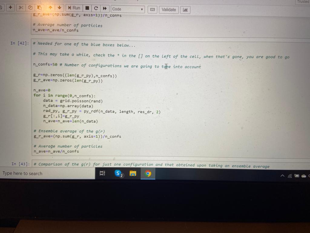
Trusted + * B A Run C Code 5_r_ave-inp. sum gr, axis=1))/n_conts 2 Validate # Average number of particles n ave=n_ave/n confs In [42]: # Needed for one of the blue boxes below… # This may take a while, check the – in the [] on the left of the cell, when that’s gone, you are good to go n_confs=5€ # Number of configurations we are going to take into account g_r=np.zeros((len(8_r_py),n_confs)) 8_r_ave=np.zeros(len(8_r_py)) n_ave=0 for i in range(e,n_confs): data = grid.poisson(rand) n_data=np.array(data) rad_py, _r_py = py_rdf(n_data, length, res_dr, 2) g_r[:,i]=g_r_py n_ave=n_ave+len(n_data) # Ensemble average of the g(r) 8_r_ave=(np.sum(@_r, axis-1)/n_confs # Average number of particles n_ave=n_ave/n_confs In [43]: # Comparison of the g(r) for just one configuration and that obtained upon taking an ensemble average Type here to search
+ 8 N Run O C Code Validate will In [43]: # Comparison of the g(r) for just one configuration and that obtained upon taking an ensemble average f_cub_ave = interpid(rad_py, g_r_ave, kind=’cubic’) xnew = np.linspace(safe, (length/2.0)-safe, num=res, endpoint=True) pit.figure(figsize=(6, 6), dpi= 8e, facecolor=’w’, edgecolor=’k’) # figsize determine the actual size of the figure plt.tick_params (axis=’both’, which=’both’, length=10., labelleft=True, labelbottom=True, labelsize=20.8) plt.plot(xnew, f_cub(xnew), color=’blue’, linestyle=’solid’, linewidth=1.0, label=’One configuration) plt.plot(xnew, f_cub_ave(xnew), color=’purple’, linestyle=’solid’, linewidth=3.0, label=’Ensemble average’) plt.xlabel(‘r [SAA$]’, fontsize=26) plt.ylabel(‘g(r)’, fontsize=26) plt.legend() plt.show() One configuration Ensemble average g(r) 0.5 L Type here to search
Run Ic Code Validate One configuration Ensemble average 2.5 2.0 1.5 g(r) 0.5 l woman 0.0 2.5 7.5 10.0 5.0 r[Å] Type here to search

Expert Answer

Answer to Use python to compute step1-4 (I already compute step1-3 and it is correct, the code of step 1-3 are shown at the pictur…

Use Python Find Way Make Period 2 Spike Instead Individual Spikes See Original Code Brian Q43782545

(Use Python) Find a way to make a period 2 spike (instead ofindividual spikes).

See original code below-

from brian2 import *

# Parameters
C = 281 * pF
gL = 30 * nS
taum = C / gL
EL = -70.6 * mV
VT = -50.4 * mV
DeltaT = 2 * mV
Vcut = VT + 5 * DeltaT

# Pick an electrophysiological behaviour
tauw, a, b, Vr = 144*ms, 20*nS, 0.0805*nA, -70.6*mV # Regularspiking (as in the paper)
#tauw,a,b,Vr=20*ms,4*nS,0.5*nA,VT+5*mV # Bursting
#tauw,a,b,Vr=144*ms,2*C/(144*ms),0*nA,-70.6*mV # Fast spiking

eqs = “””
dvm/dt = (gL*(EL – vm) + gL*DeltaT*exp((vm – VT)/DeltaT) + I – w)/C: volt
dw/dt = (a*(vm – EL) – w)/tauw : amp
I : amp
“””

neuron = NeuronGroup(1, model=eqs, threshold=’vm>Vcut’,
reset=”vm=Vr; w+=b”, method=’euler’)
neuron.vm = EL
trace = StateMonitor(neuron, ‘vm’, record=0)
spikes = SpikeMonitor(neuron)

run(20 * ms)
neuron.I = 1*nA
run(100 * ms)
neuron.I = 0*nA
run(20 * ms)

# We draw nicer spikes
vm = trace[0].vm[:]
for t in spikes.t:
i = int(t / defaultclock.dt)
vm[i] = 20*mV

fig, ax = plt.subplots()
# Using set_dashes() to modify dashing of an existing line
line1, = ax.plot(trace.t / ms, vm / mV, label=’Basic Spike’)
#line1.set_dashes([2, 2, 10, 2]) # 2pt line, 2pt break, 10pt line,2pt break
ax.legend()
plt.show()

Expert Answer

Answer to (Use Python) Find a way to make a period 2 spike (instead of individual spikes). See original code below- from brian2 im…

Use Python Part1 Https Wwwcheggcom Homework Help Questions Answers 21 Experimental Analysi Q43863726

use python:

Part1:https://www.chegg.com/homework-help/questions-and-answers/21-experimental-analysis-part-1-common-loop-appears-programming-problems-partial-double-lo-q38816417

Part2:https://www.chegg.com/homework-help/questions-and-answers/22-experimental-analysis-part-2-many-functions-look-defined-recursively-merge-sort-general-q38828542

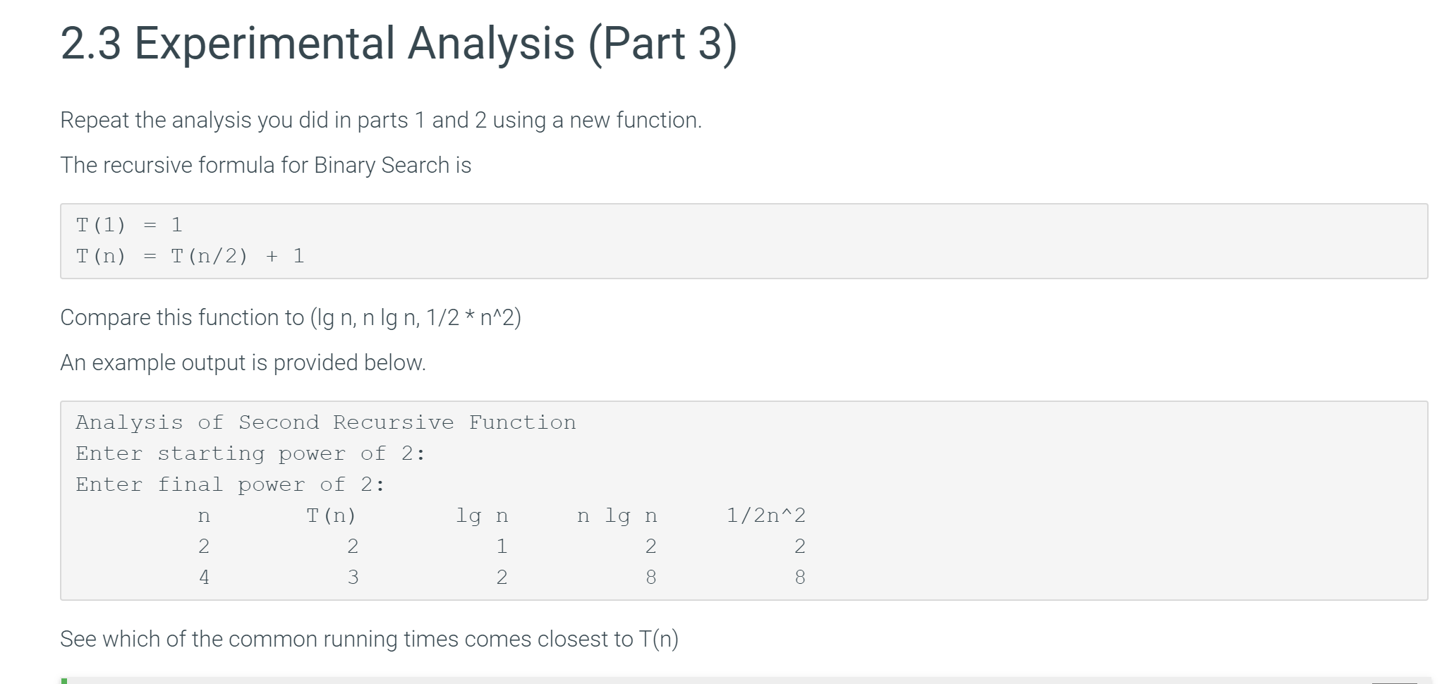
2.3 Experimental Analysis (Part 3) Repeat the analysis you did in parts 1 and 2 using a new function. The recursive formula for Binary Search is T (1) T(n) = 1 = T (n/2) + 1 Compare this function to (Ig n, n Ign, 1/2 * n^2) An example output is provided below. Analysis of Second Recursive Function Enter starting power of 2: Enter final power of 2: T (n) lg n n lg n 1/2n^2 s N Nm 00 See which of the common running times comes closest to T(n) Show transcribed image text 2.3 Experimental Analysis (Part 3) Repeat the analysis you did in parts 1 and 2 using a new function. The recursive formula for Binary Search is T (1) T(n) = 1 = T (n/2) + 1 Compare this function to (Ig n, n Ign, 1/2 * n^2) An example output is provided below. Analysis of Second Recursive Function Enter starting power of 2: Enter final power of 2: T (n) lg n n lg n 1/2n^2 s N Nm 00 See which of the common running times comes closest to T(n)

Expert Answer

Answer to use python: Part1: https://www.chegg.com/homework-help/questions-and-answers/21-experimental-analysis-part-1-common-loop…

Use Python Part1 Https Wwwcheggcom Homework Help Questions Answers 21 Experimental Analysi Q43869110

use python:

Part1:https://www.chegg.com/homework-help/questions-and-answers/21-experimental-analysis-part-1-common-loop-appears-programming-problems-partial-double-lo-q38816417

Part2:https://www.chegg.com/homework-help/questions-and-answers/22-experimental-analysis-part-2-many-functions-look-defined-recursively-merge-sort-general-q38828542

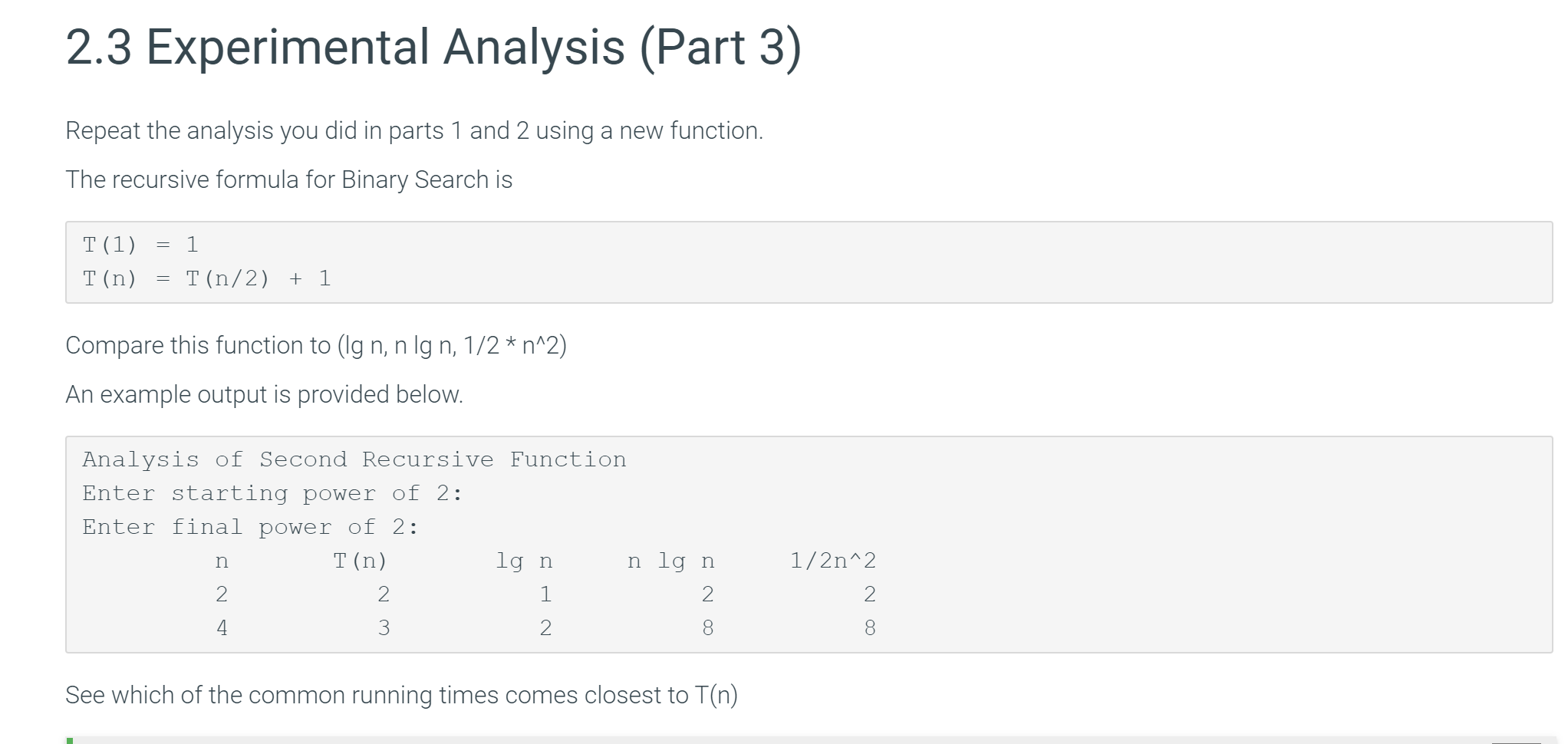
2.3 Experimental Analysis (Part 3) Repeat the analysis you did in parts 1 and 2 using a new function. The recursive formula for Binary Search is T (1) T(n) = 1 = T (n/2) + 1 Compare this function to (Ig n, n Ign, 1/2 * n^2) An example output is provided below. Analysis of Second Recursive Function Enter starting power of 2: Enter final power of 2: T (n) lg n n lg n 1/2n^2 s N Nm 00 See which of the common running times comes closest to T(n) Show transcribed image text 2.3 Experimental Analysis (Part 3) Repeat the analysis you did in parts 1 and 2 using a new function. The recursive formula for Binary Search is T (1) T(n) = 1 = T (n/2) + 1 Compare this function to (Ig n, n Ign, 1/2 * n^2) An example output is provided below. Analysis of Second Recursive Function Enter starting power of 2: Enter final power of 2: T (n) lg n n lg n 1/2n^2 s N Nm 00 See which of the common running times comes closest to T(n)

Expert Answer

Answer to use python: Part1: https://www.chegg.com/homework-help/questions-and-answers/21-experimental-analysis-part-1-common-loop…

Use Quantize Function Python Round Answers Nearest Whole Number Someone Help Fix Code Get Q43783006

How do I use the quantize function in python to round my answersto the nearest whole number? Can someone help me fix the code so Ican get all my answers rounded to the nearest whole number? Also isit possible to take out duplicates in the answer?

Here is the code:

#importing xlwt library to write into xls
import xlwt
from xlwt import Workbook

#create a workbook
wb = Workbook()
#create a sheet
sheet = wb.add_sheet(‘Sheet’)

#percentages list
percentages = [23.6, 38.2, 50, 61.8, 78.6, 113, 123.6, 138.2,161.8]
#add first row
for i in range(len(percentages)):
   sheet.write(0,i+1,str(percentages[i])+’%’)

#user input
n = int(input(‘Enter number of elements: ‘))
#second row starts from index 1
row=1
print(‘Enter numbers: ‘)
for i in range(n):
    #User input
   val = float(input())
   #Add entered value to first column of the row
   sheet.write(row,0,str(val))
   #calculate each percentage
   for j in range(len(percentages)):
       result =(percentages[j]/100)*val
       #write result to sheet by roundingupto 3 decimal points
      sheet.write(row,j+1,str(round(result,3)))
   #increment the row by 1
   row+=1
#save Workbook as xls`
wb.save(‘percentages.xls’)

Expert Answer

Answer to How do I use the quantize function in python to round my answers to the nearest whole number? Can someone help me fix th…

Use Quick Sort Method Discussed Note Video Clip Sort Following Items Given Order Display S Q43805177

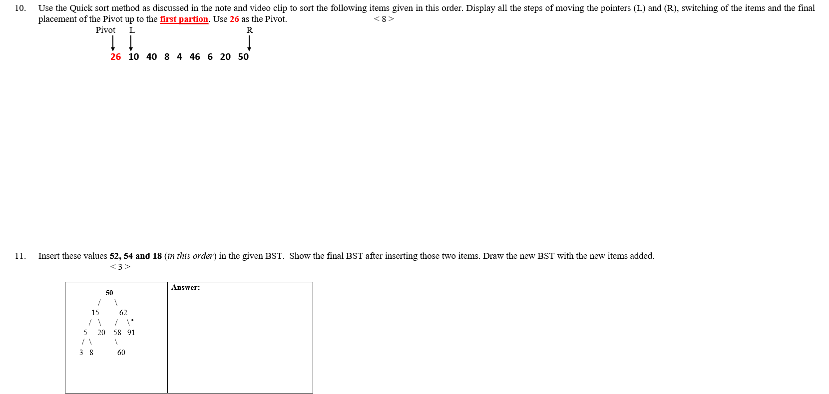
Use the Quick sort method as discussed in the note and video clip to sort the following items given in this order. Display all the steps of moving the pointers (L) and (R), switching of the items and the final placement of the Pivot up to the first partion. Use 26 as the Pivot. 10. <8> Pivot 26 10 40 8 4 46 6 20 50 Insert these values 52, 54 and 18 (in this order) in the given BST. Show the final BST after inserting those two items. Draw the new BST with the new items added. 11. < 3 > Answer: 50 15 62 20 58 91 3 8 60 Show transcribed image text Use the Quick sort method as discussed in the note and video clip to sort the following items given in this order. Display all the steps of moving the pointers (L) and (R), switching of the items and the final placement of the Pivot up to the first partion. Use 26 as the Pivot. 10. Pivot 26 10 40 8 4 46 6 20 50 Insert these values 52, 54 and 18 (in this order) in the given BST. Show the final BST after inserting those two items. Draw the new BST with the new items added. 11. Answer: 50 15 62 20 58 91 3 8 60

Expert Answer

Answer to Use the Quick sort method as discussed in the note and video clip to sort the following items given in this order. Displ…

Use Relevant Examples Discuss Concept Local Static Variables Visual Basic Oop Edp Q43809035(1)

With the use of relevant examples discuss the concept local andstatic variables in Visual Basic (OOP and EDP)

Expert Answer

Answer to With the use of relevant examples discuss the concept local and static variables in Visual Basic (OOP and EDP)…

Use Relevant Examples Discuss Concept Local Static Variables Visual Basic Oop Edp Q43809035

With the use of relevant examples discuss the concept local andstatic variables in Visual Basic (OOP and EDP)

Expert Answer

Answer to With the use of relevant examples discuss the concept local and static variables in Visual Basic (OOP and EDP)…