Newton S Method Matlab Module Going Use Newton S Method Compute Root S Function F X X 3×2 Q43818011

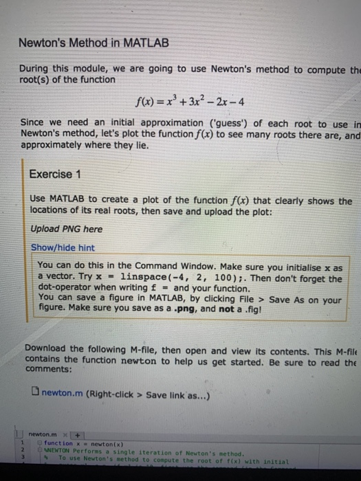
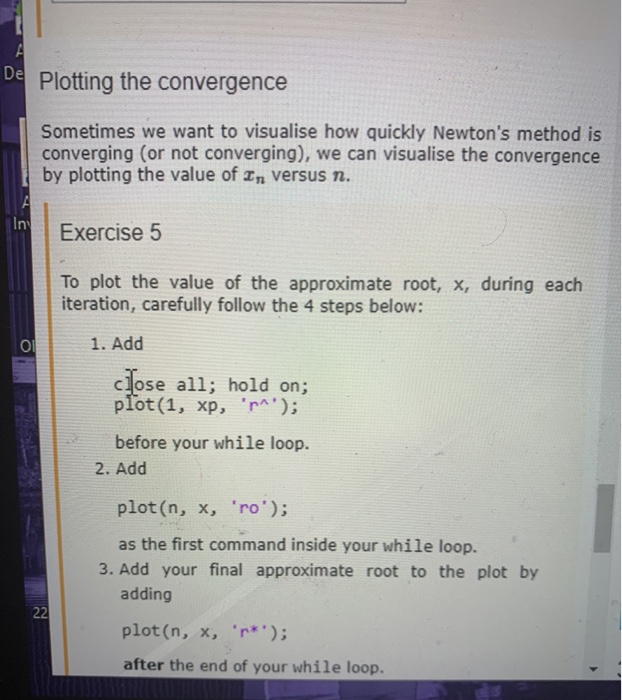
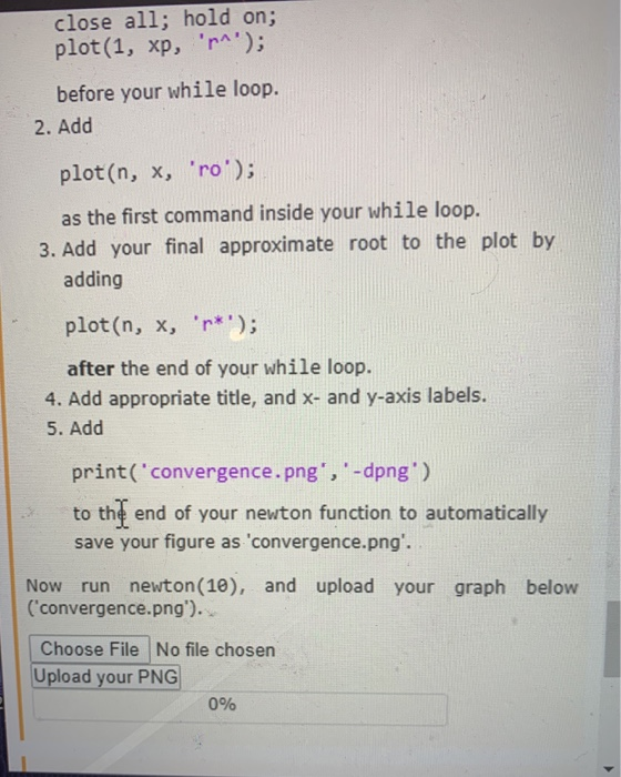
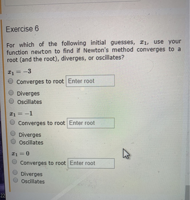Newtons Method in MATLAB During this module, we are going to use Newtons method to compute the root(s) of the function f(x) Newton’s Method in MATLAB During this module, we are going to use Newton’s method to compute the root(s) of the function f(x) = x + 3×2 – 2x – 4 Since we need an initial approximation (‘guess’) of each root to use in Newton’s method, let’s plot the function f(x) to see many roots there are, and approximately where they lie. Exercise 1 Use MATLAB to create a plot of the function f(x) that clearly shows the locations of its real roots, then save and upload the plot: Upload PNG here Show/hide hint You can do this in the Command Window. Make sure you initialise x as a vector. Try x =linspace(-4, 2, 100);. Then don’t forget the dot-operator when writing f = and your function. You can save a figure in MATLAB, by clicking File > Save As on your figure. Make sure you save as a .png, and not a .fig! Download the following M-file, then open and view its contents. This M-file contains the function newton to help us get started. Be sure to read the comments: newton.m (Right click > Save link as…) newton. m x + 1 function X = newtonix) WEWTON Performs a single iteration of Newton’s method. To use Newton’s ethod to compute the root off with initial 2 newton.m (Right-click > Save link as…) newton. m x + function x = newton(x) NEWTON Performs a single iteration of Newton’s method. To use Newton’s method to compute the root of f(x) with initial guess x1, e.g. if x1 is 10, first use the command (in the Command Window): x = newton (10) to compute the next approximate root. Then further approximate roots are computed by repeatedly executing the command: x = newton(x) 16 – Perform one iteration of Newton’s method. n = 2; computed after 1 interation (not really needed until exe! xp = x; % xp is “x-previous” and contains x1 X = xp – f(xp)/fprime(xp); x is the next x being computed, X2 Exercise 3 add while loop here alternative to ‘disp’ function – keeps things neat! fprintf(“Newton approximates root at *.15f, after ad iter fprintf(‘f(x) at approximate root xis 1.6fn’, f(x)); fprintf(“x-xplis 1.6f’, abs(x-xp)); End of function. end 25 26 – 29 38 – 31 – To change the function f(x), edit this function. function y = f(x) y = x^3 + 3*x^2 – 2x – 4; end 34 35 – 36 – To change the function f'(x), edit this function. function yprime – fprime(x) yprime = 3*x^2 + 6 x – 2; end Exercise 2 Your plot from Exercise 1 should show that f(x) has a root near x = 1.23. Use the function newton with initial guess x1 = 10, to compute an approximation of this root by computing successive approximate roots X2, X3, X4, … until xn – Xn-11 < 10- for the first time. Enter the values X2, X3, X4,… that you computed (in order, and separated by commas): Enter approximate roots Enter the value of x-xp when it is less than 10 or 0.001, for the first time (copy-paste exact value shown from running newton: |x-xp is Enter the value of f(x) when Ix-xpl < 10-‘ for the first time: Enter computed value Show/hide hint Exercise 3 Add a while loop to newton.m iterations of Newton’s method. that performs additional 1. Your loop should run while lx – xpl 10-3 is true. 2. n should be incremented by 1 every loop. Exercise 3 Add a while loop to newton.m that performs additional iterations of Newton’s method. 1. Your loop should run while Ix – xpl> 10-is true. 2. n should be incremented by 1 every loop. 3. Don’t forget to re-calculate xp and x every loop! Check that your while loop is working correctly. Type >> newton (10); into the Command Window and check if it outputs: Newton approximates root at 1.236067979714056, after 8 iteration(s) f(x) at approximate root x is 0.000000 | x-xplis 0.000057 Use the following prompt to upload newton.m: Browse… No file selected. Upload your M-file 0% Newton’s method is not a fail-safe way to find roots, since the sequence of approximations may not converge for a ‘bad’ initial guess. This is a downside of Newton’s method (compared to the Bisection method, which will always converge for valid initial values). ULLII CUB of iterations. If a ‘bad guess is made, this is stop the while loop Tom looping forever. For this, we need to insert a counter into the while loop to keep track of how many iterations have passed. Exercise 4 Add an extra condition to your while loop, so that the loop will exit once n is greater than 101. Hint: Use &&. Show/hide hint Here is a very simple example of having multiple conditions for a while loop. a = 17 b = 1; while a < 10 && b < 20 % do something with a and b end If either a, or b, become a value other than 1, the while loop condition will fail, and the program will exit the loop and continue executing any code below it. How many iterations does it take to find the approximate root, for initial guess Ij = 1? Enter iterations 22 De Plotting the convergence Sometimes we want to visualise how quickly Newton’s method is converging (or not converging), we can visualise the convergence by plotting the value of In versus n. Exercise 5 To plot the value of the approximate root, x, during each iteration, carefully follow the 4 steps below: 1. Add close all; hold on; plot(1, xp, ‘p^’); before your while loop. 2. Add plot(n, x, ‘ro’); as the first command inside your while loop. 3. Add your final approximate root to the plot by! adding plot(n, X, ‘*’); after the end of your while loop. close all; hold on; plot(1, xp, ‘^’); before your while loop. 2. Add plot(n, x, ‘ro’); as the first command inside your while loop. 3. Add your final approximate root to the plot by adding plot(n, X, ‘*’); after the end of your while loop. 4. Add appropriate title, and X- and y-axis labels. 5. Add print(‘convergence.png’,’-dpng’) to the end of your newton function to automatically save your figure as ‘convergence.png’. Now run newton(10), and upload your graph below (‘convergence.png’). Choose File No file chosen Upload your PNG 0% Exercise 6 For which of the following initial guesses, Ii, use your function newton to find if Newton’s method converges to a root (and the root), diverges, or oscillates? I1= -3 Converges to root Enter root O Diverges Oscillates Ij = -1 Converges to root Enter root Diverges Oscillates Il=0 O Converges to root Enter root Diverges Oscillates 22 Show transcribed image text Newton’s Method in MATLAB During this module, we are going to use Newton’s method to compute the root(s) of the function f(x) = x + 3×2 – 2x – 4 Since we need an initial approximation (‘guess’) of each root to use in Newton’s method, let’s plot the function f(x) to see many roots there are, and approximately where they lie. Exercise 1 Use MATLAB to create a plot of the function f(x) that clearly shows the locations of its real roots, then save and upload the plot: Upload PNG here Show/hide hint You can do this in the Command Window. Make sure you initialise x as a vector. Try x =linspace(-4, 2, 100);. Then don’t forget the dot-operator when writing f = and your function. You can save a figure in MATLAB, by clicking File > Save As on your figure. Make sure you save as a .png, and not a .fig! Download the following M-file, then open and view its contents. This M-file contains the function newton to help us get started. Be sure to read the comments: newton.m (Right click > Save link as…) newton. m x + 1 function X = newtonix) WEWTON Performs a single iteration of Newton’s method. To use Newton’s ethod to compute the root off with initial 2
newton.m (Right-click > Save link as…) newton. m x + function x = newton(x) NEWTON Performs a single iteration of Newton’s method. To use Newton’s method to compute the root of f(x) with initial guess x1, e.g. if x1 is 10, first use the command (in the Command Window): x = newton (10) to compute the next approximate root. Then further approximate roots are computed by repeatedly executing the command: x = newton(x) 16 – Perform one iteration of Newton’s method. n = 2; computed after 1 interation (not really needed until exe! xp = x; % xp is “x-previous” and contains x1 X = xp – f(xp)/fprime(xp); x is the next x being computed, X2 Exercise 3 add while loop here alternative to ‘disp’ function – keeps things neat! fprintf(“Newton approximates root at *.15f, after ad iter fprintf(‘f(x) at approximate root xis 1.6fn’, f(x)); fprintf(“x-xplis 1.6f’, abs(x-xp)); End of function. end 25 26 – 29 38 – 31 – To change the function f(x), edit this function. function y = f(x) y = x^3 + 3*x^2 – 2x – 4; end 34 35 – 36 – To change the function f'(x), edit this function. function yprime – fprime(x) yprime = 3*x^2 + 6 x – 2; end
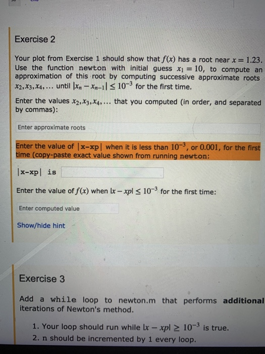
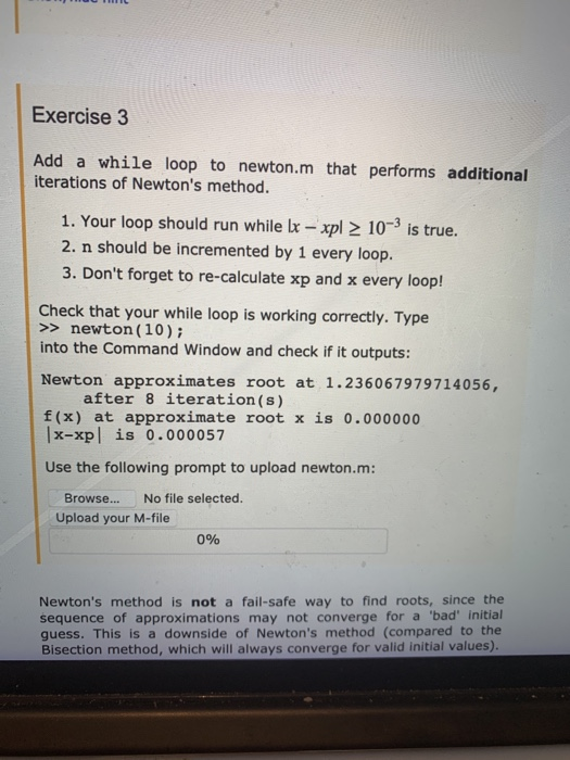
Exercise 2 Your plot from Exercise 1 should show that f(x) has a root near x = 1.23. Use the function newton with initial guess x1 = 10, to compute an approximation of this root by computing successive approximate roots X2, X3, X4, … until xn – Xn-11 > newton (10); into the Command Window and check if it outputs: Newton approximates root at 1.236067979714056, after 8 iteration(s) f(x) at approximate root x is 0.000000 | x-xplis 0.000057 Use the following prompt to upload newton.m: Browse… No file selected. Upload your M-file 0% Newton’s method is not a fail-safe way to find roots, since the sequence of approximations may not converge for a ‘bad’ initial guess. This is a downside of Newton’s method (compared to the Bisection method, which will always converge for valid initial values).
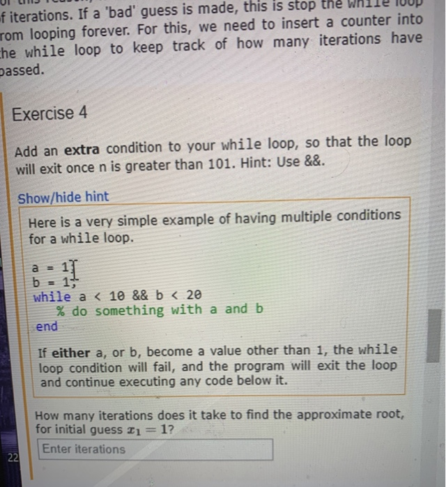
ULLII CUB of iterations. If a ‘bad guess is made, this is stop the while loop Tom looping forever. For this, we need to insert a counter into the while loop to keep track of how many iterations have passed. Exercise 4 Add an extra condition to your while loop, so that the loop will exit once n is greater than 101. Hint: Use &&. Show/hide hint Here is a very simple example of having multiple conditions for a while loop. a = 17 b = 1; while a