(Solved) : Grader Instructions Excel 2016 Project Ex16 Xl Comp Grader Cap Manufacturing 15 Project De Q37295658 . . .
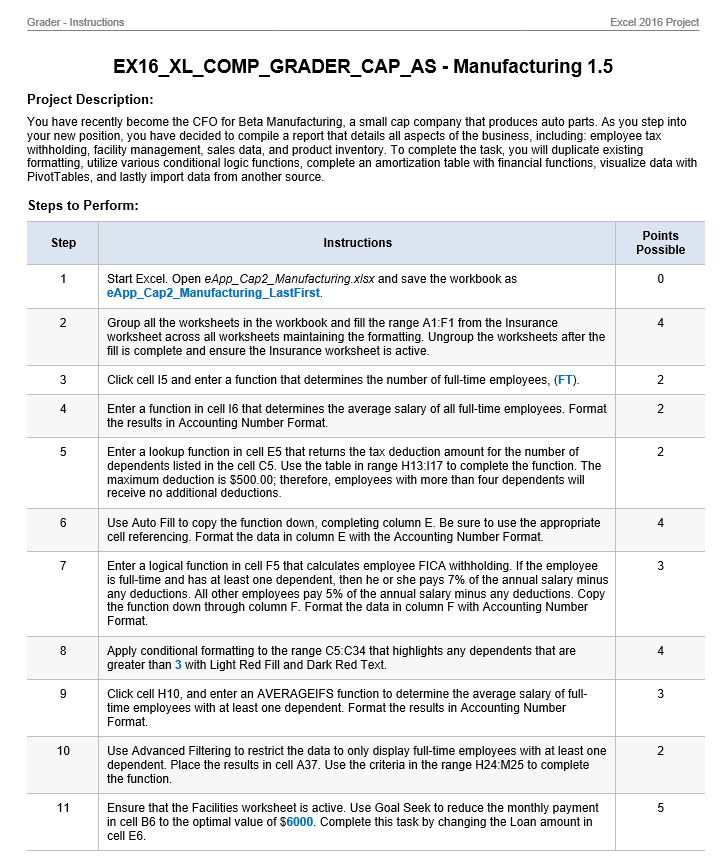
Grader- Instructions Excel 2016 Project EX16 XL COMP GRADER CAP AS – Manufacturing 1.5 Project Description: You have recently become the CFO for Beta Manufacturing, a small cap company that produces auto parts. As you step into your new position, you have decided to compile a report that details all aspects of the business, including employee tax withholding, facility management, sales data, and product inventory. To complete the task, you will duplicate existing formatting, utilize various conditional logic functions, complete an amortization table with financial functions, visualize data with PivotTables, and lastly import data from another source Steps to Perform: Points Possible Step Instructions Start Excel. Open eApp Cap2_Manufacturing xisx and save the workbook as eAppCap2Manufacturing_LastFirst. Group all the worksheets in the workbook and fill the range A1:F1 from the Insurance worksheet across all worksheets maintaining the formatting. Ungroup the worksheets after the fill is complete and ensure the Insurance worksheet is active 4 Click cell 15 and enter a function that determines the number of full-time employees, (FT). Enter a function in cell 16 that determines the average salary of all full-time employees. Format the results in Accounting Number Format. Enter a lookup function in cell E5 that returns the tax deduction amount for the number of dependents listed in the cell C5. Use the table in range H13:117 to complete the function. The maximum deduction is $500.00, therefore, employees with more than four dependents will receive no additional deductions Use Auto Fill to copy the function down, completing column E. Be sure to use the appropriate cell referencing. Format the data in column E with the Accounting Number Format. 4 Enter a logical function in cell F5 that calculates employee FICA withholding. If the employee is full-time and has at least one dependent, then he or she pays 7% of the annual salary minus any deductions. All other employees pay 5% of the annual salary minus any deductions. Copy the function down through column F. Format the data in column F with Accounting Number Format. Apply conditional formatting to the range C5:C34 that highlights any dependents that are greater than 3 with Light Red ill and Dark Red Text. 4 Click cell H10, and enter an AVERAGEIFS function to determine the average salary of full time employees with at least one dependent. Format the results in Accounting Number Format. 10 Use Advanced Filtering to restrict the data to only display full-time employees with at least one dependent. Place the results in cell A37. Use the criteria in the range H24:M25 to complete the function Ensure that the Facilities worksheet is active. Use Goal Seek to reduce the monthly payment in cell B6 to the optimal value of $6000. Complete this task by changing the Loan amount in cell E6 Points Possible Step Instructions Create the following three scenarios using Scenario Manager. The scenarios should change the cells B7, B8, and E6 B7 .0325 E6 275000 Most Likely B7 .057 E6 312227.32 Bad B7 ,0700 E6- 350000 Create a Scenario Summary Report based on the value in cell B6. Format the new report appropriately 13 Ensure that the Facilities worksheet is active. Enter a reference to the beginning loan balance in cell B12 and enter a reference to the payment amount in cell C12. 4 14 Enter a function in cell D12, based on the payment and loan details, that calculates the amount of interest paid on the first payment. Be sure to use the appropriate absolute, relative or mixed cell references 15 Enter a function in cell E12, based on the payment and loan details, that calculates the amount of principal paid on the first payment. Be sure to use the appropriate absolute, relative or mixed cell references 16 Enter a formula in cell F12 to calculate the remaining balance after the current payment. The remaining balance is calculated by subtracting the principal payment from the balance in column B Enter a function in cell G12, based on the payment and loan details, that calculates the amount of cumulative interest paid on the first payment Be sure to use the appropriate absolute, relative, or mixed cell references 18 Enter a function in cell H12, based on the payment and loan details, that calculates the amount of cumulative principal paid on the first payment. Be sure to use the appropriate absolute, relative, or mixed cell references Enter a reference to the remaining balance of payment 1 in cell B13. Use the fill handle to copy the functions created in the prior steps down to complete the amortization table 20 Ensure the Sales worksheet is active. Enter a function in cell B8 to create a custom transaction number. The transaction number should be comprised of the item number listed in cell C8 combined with the quantity in cell D8 and the first initial of the payment type in cell E8 Use Auto Fill to copy the function down, completing the data in column B 21 Enter a nested function in cell G8 that displays the word Flag if the Payment Type is Credit and the Amount is greater than or equal to $4000. Otherwise, the function will display a blank cell. Use Auto Fill to copy the function down, completing the data in column G. Points Possible Step Instructions Create a data validation list in cell D5 that displays Quantity, Payment Type, and Amount. Type the Trans# 30038C in cell B5, and select Quantity from the validation list in cell D5 Enter a nested lookup function in cell F5 that evaluates the Trans # in cell B5 as well as the Category in cell D5, and returns the results based on the data in the range A8:F32. 25 Create a PivotTable based on the range A7:G32. Place the PivotTable in cell 117 on the current worksheet. Place Payment Type in the Rows box and Amount in the Values box. Format the Amount with Accounting Number Format. 26 Insert a PivotChart using the Pie chart type based on the data. Place the upper-left corner of the chart inside cell 122. Format the Legend of the chart to appear at the bottom of the chart area. Format the Data Labels to appear on the Outside end of the chart. 4 Note, Mac users, select the range 118:J20, on the Insert tab, click Recommended Charts, and then click Pie. Format the legend, and apply the data labels as specified 27 Insert a Slicer based on Date. Place the upper-left corner of the Slicer inside cell L8 28 Ensure the Inventory worksheet is active. Import the Access database eApp_Cap2_Inventory.accab into the worksheet starting in cell A3 Note, Mac users, download and import the delimited Inventory.txt file into the worksheet starting in cell A3 29 Create a footer with your name on the left, the sheet code in the center, and the file name on the right for each worksheet. 30 Save and close the file. Based on your instructor’s directions, submit eApp_Cap2_Manufacturing_LastFirst.xlsx 100 Total Points A1 Facility Amortization Table Payment Details Loan Details $6,245.45 325,000.00 6 Payment 7 APR 8 Years 9 Pmts per Year Loan Periodic Rate # of Payments 5.75% 0.479% 12 Payment Beginning Payment Number Principal Remaining Cumulative Cumulative BalanceAmount Interest Paid Repayment Balance Principal Interest 12 2 16 17 18 19 10 23 12 13 14 15 16 17 18 19 25 27 30 32 21 23 24 25 2б 37 Insurance Facilities Sales Inventory 2 2 1|2|3 xFICA Withholdings H19 0 Beta Manufacturing Emplo e Withholdings 4 Employee ID Status Dependents Salary Deduction Withholding Statistics $ 90,212 $ 18,984 $ 42,906 $ 37,191 $52,528 $ 17,126 $ 94,101 $ 12,471 $67,132 $ 88,604 $55,680 $ 98,869 $11,994 S 17,957 $66,693 $ 84,432 $18,994 $ 65,648 $ 18,835 $ 15,525 $ 15,861 $ 16,173 $9,893 $17,081 S 39,364 $19,306 S 9,933 $16,707 S 13,665 $7,688 Number of FT Employees Average Salary Full Time 7276 FT 9858 P 8936 FT 6881 FT 3852 FT 6580 PT 4772 FT 4296 PT 8884 FT 9916 FT 5803 FT 8708 FT 5565 PT 6142 PT 8164 FT 4338 FT 5833 PT 6060 FT 2559 PT 5569 PT 3488 PT 7353 PT 4990 P 4785 PT 3040 FT 8087 PT 4474 PT 4251 PT 5324 PT 3123 PT Additional Information Average Salary of FT 1 Dependent Dependents Deduction 50.00 S 125.00 250.00 S 325.00 $500.00 14 15 FICA Withholdin 19 FT at least 1 Dependent PT or FT No De 5% ents 23 Employee ID Status Dependents Salary Deduction Withholdings FT 25 26 27 28 29 31 35 37 Insurance Facilities Sales Inventory XVfcResults E5 March Transactions Search Results 4 Results 5 Trans # Categor Date Trans # Item Quantity Payment Type Amount status $4,800 $2,800 8 3/1/2018 93/2/2018 10 3/3/2018 11 3/3/2018 12 3/5/2018 13 3/7/2018 14 3/9/2018 15 3/10/2018 16 3/10/2018 17 3/10/2018 18 3/11/2018 19 3/11/2018 20 3/12/2018 21 3/13/2018 22 3/13/2018 23 3/14/2018 24 3/18/2018 25 3/24/2018 26 3/24/2018 27 3/24/2018 28 3/28/2018 29 3/28/2018 30 3/30/2018 31 3/30/2018 32 3/30/2018 3003 Credit 4Financed 1 Credit 10 Financed $7,000 $1,500 $3,500 $1,250 $2,100 Credit 1001 5 Credit 5 Credit 3 Credit 1 Financed 4Financed 9 Financed 1001 2002 $2,600 $4,500 $4,800 $2,250 $4,000 $4,500 2002 3003 1001 2002 2002 3003 3003 Credit 9 Financed 8 Financed Credit Credit 9 1 Credit 1 Credit 3 Financed $1,950 $6,500 $5,000 $2,250 $4,800 $3,900 $4,500 10 10 Cash Credit Cash Credit 2002 1001 3003 6 Financed Cash 2002 Inventory – Notepad File Edit Format View Help Item Quantity 002 3500 35000 A 003 2500 30000B 0044000 22000 C 5005 1000 18000 D Total Value Warehouse1001 5000 40000 A Show transcribed image text Grader- Instructions Excel 2016 Project EX16 XL COMP GRADER CAP AS – Manufacturing 1.5 Project Description: You have recently become the CFO for Beta Manufacturing, a small cap company that produces auto parts. As you step into your new position, you have decided to compile a report that details all aspects of the business, including employee tax withholding, facility management, sales data, and product inventory. To complete the task, you will duplicate existing formatting, utilize various conditional logic functions, complete an amortization table with financial functions, visualize data with PivotTables, and lastly import data from another source Steps to Perform: Points Possible Step Instructions Start Excel. Open eApp Cap2_Manufacturing xisx and save the workbook as eAppCap2Manufacturing_LastFirst. Group all the worksheets in the workbook and fill the range A1:F1 from the Insurance worksheet across all worksheets maintaining the formatting. Ungroup the worksheets after the fill is complete and ensure the Insurance worksheet is active 4 Click cell 15 and enter a function that determines the number of full-time employees, (FT). Enter a function in cell 16 that determines the average salary of all full-time employees. Format the results in Accounting Number Format. Enter a lookup function in cell E5 that returns the tax deduction amount for the number of dependents listed in the cell C5. Use the table in range H13:117 to complete the function. The maximum deduction is $500.00, therefore, employees with more than four dependents will receive no additional deductions Use Auto Fill to copy the function down, completing column E. Be sure to use the appropriate cell referencing. Format the data in column E with the Accounting Number Format. 4 Enter a logical function in cell F5 that calculates employee FICA withholding. If the employee is full-time and has at least one dependent, then he or she pays 7% of the annual salary minus any deductions. All other employees pay 5% of the annual salary minus any deductions. Copy the function down through column F. Format the data in column F with Accounting Number Format. Apply conditional formatting to the range C5:C34 that highlights any dependents that are greater than 3 with Light Red ill and Dark Red Text. 4 Click cell H10, and enter an AVERAGEIFS function to determine the average salary of full time employees with at least one dependent. Format the results in Accounting Number Format. 10 Use Advanced Filtering to restrict the data to only display full-time employees with at least one dependent. Place the results in cell A37. Use the criteria in the range H24:M25 to complete the function Ensure that the Facilities worksheet is active. Use Goal Seek to reduce the monthly payment in cell B6 to the optimal value of $6000. Complete this task by changing the Loan amount in cell E6
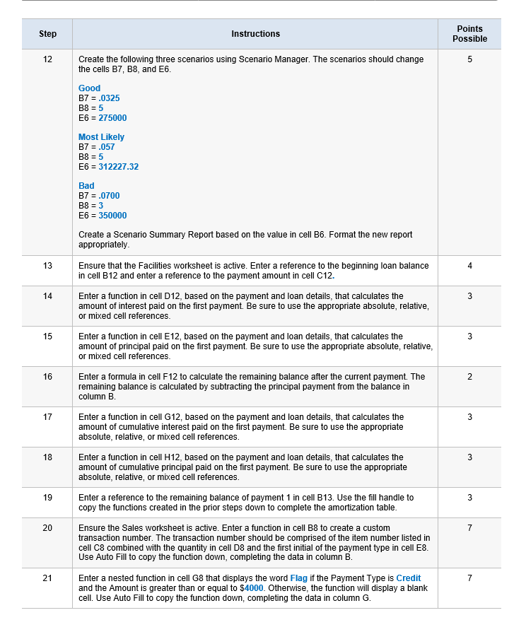
Points Possible Step Instructions Create the following three scenarios using Scenario Manager. The scenarios should change the cells B7, B8, and E6 B7 .0325 E6 275000 Most Likely B7 .057 E6 312227.32 Bad B7 ,0700 E6- 350000 Create a Scenario Summary Report based on the value in cell B6. Format the new report appropriately 13 Ensure that the Facilities worksheet is active. Enter a reference to the beginning loan balance in cell B12 and enter a reference to the payment amount in cell C12. 4 14 Enter a function in cell D12, based on the payment and loan details, that calculates the amount of interest paid on the first payment. Be sure to use the appropriate absolute, relative or mixed cell references 15 Enter a function in cell E12, based on the payment and loan details, that calculates the amount of principal paid on the first payment. Be sure to use the appropriate absolute, relative or mixed cell references 16 Enter a formula in cell F12 to calculate the remaining balance after the current payment. The remaining balance is calculated by subtracting the principal payment from the balance in column B Enter a function in cell G12, based on the payment and loan details, that calculates the amount of cumulative interest paid on the first payment Be sure to use the appropriate absolute, relative, or mixed cell references 18 Enter a function in cell H12, based on the payment and loan details, that calculates the amount of cumulative principal paid on the first payment. Be sure to use the appropriate absolute, relative, or mixed cell references Enter a reference to the remaining balance of payment 1 in cell B13. Use the fill handle to copy the functions created in the prior steps down to complete the amortization table 20 Ensure the Sales worksheet is active. Enter a function in cell B8 to create a custom transaction number. The transaction number should be comprised of the item number listed in cell C8 combined with the quantity in cell D8 and the first initial of the payment type in cell E8 Use Auto Fill to copy the function down, completing the data in column B 21 Enter a nested function in cell G8 that displays the word Flag if the Payment Type is Credit and the Amount is greater than or equal to $4000. Otherwise, the function will display a blank cell. Use Auto Fill to copy the function down, completing the data in column G.
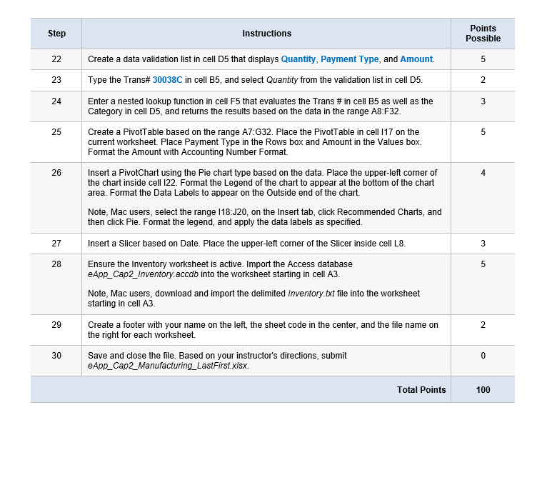
Points Possible Step Instructions Create a data validation list in cell D5 that displays Quantity, Payment Type, and Amount. Type the Trans# 30038C in cell B5, and select Quantity from the validation list in cell D5 Enter a nested lookup function in cell F5 that evaluates the Trans # in cell B5 as well as the Category in cell D5, and returns the results based on the data in the range A8:F32. 25 Create a PivotTable based on the range A7:G32. Place the PivotTable in cell 117 on the current worksheet. Place Payment Type in the Rows box and Amount in the Values box. Format the Amount with Accounting Number Format. 26 Insert a PivotChart using the Pie chart type based on the data. Place the upper-left corner of the chart inside cell 122. Format the Legend of the chart to appear at the bottom of the chart area. Format the Data Labels to appear on the Outside end of the chart. 4 Note, Mac users, select the range 118:J20, on the Insert tab, click Recommended Charts, and then click Pie. Format the legend, and apply the data labels as specified 27 Insert a Slicer based on Date. Place the upper-left corner of the Slicer inside cell L8 28 Ensure the Inventory worksheet is active. Import the Access database eApp_Cap2_Inventory.accab into the worksheet starting in cell A3 Note, Mac users, download and import the delimited Inventory.txt file into the worksheet starting in cell A3 29 Create a footer with your name on the left, the sheet code in the center, and the file name on the right for each worksheet. 30 Save and close the file. Based on your instructor’s directions, submit eApp_Cap2_Manufacturing_LastFirst.xlsx 100 Total Points
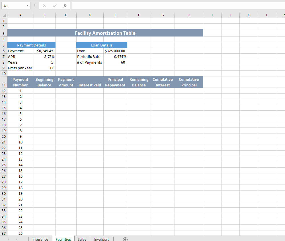
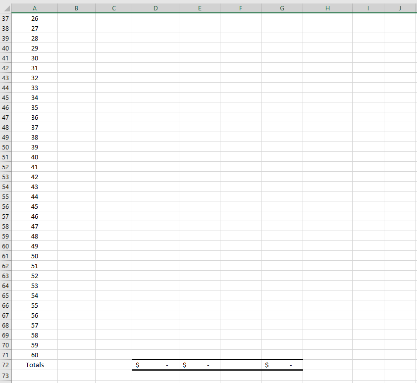
A1 Facility Amortization Table Payment Details Loan Details $6,245.45 325,000.00 6 Payment 7 APR 8 Years 9 Pmts per Year Loan Periodic Rate # of Payments 5.75% 0.479% 12 Payment Beginning Payment Number Principal Remaining Cumulative Cumulative BalanceAmount Interest Paid Repayment Balance Principal Interest 12 2 16 17 18 19 10 23 12 13 14 15 16 17 18 19 25 27 30 32 21 23 24 25 2б 37 Insurance Facilities Sales Inventory
2 2 1|2|3
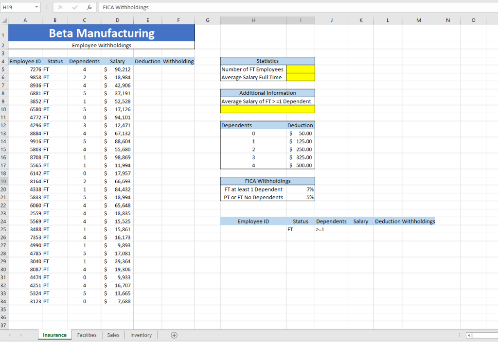
xFICA Withholdings H19 0 Beta Manufacturing Emplo e Withholdings 4 Employee ID Status Dependents Salary Deduction Withholding Statistics $ 90,212 $ 18,984 $ 42,906 $ 37,191 $52,528 $ 17,126 $ 94,101 $ 12,471 $67,132 $ 88,604 $55,680 $ 98,869 $11,994 S 17,957 $66,693 $ 84,432 $18,994 $ 65,648 $ 18,835 $ 15,525 $ 15,861 $ 16,173 $9,893 $17,081 S 39,364 $19,306 S 9,933 $16,707 S 13,665 $7,688 Number of FT Employees Average Salary Full Time 7276 FT 9858 P 8936 FT 6881 FT 3852 FT 6580 PT 4772 FT 4296 PT 8884 FT 9916 FT 5803 FT 8708 FT 5565 PT 6142 PT 8164 FT 4338 FT 5833 PT 6060 FT 2559 PT 5569 PT 3488 PT 7353 PT 4990 P 4785 PT 3040 FT 8087 PT 4474 PT 4251 PT 5324 PT 3123 PT Additional Information Average Salary of FT 1 Dependent Dependents Deduction 50.00 S 125.00 250.00 S 325.00 $500.00 14 15 FICA Withholdin 19 FT at least 1 Dependent PT or FT No De 5% ents 23 Employee ID Status Dependents Salary Deduction Withholdings FT 25 26 27 28 29 31 35 37 Insurance Facilities Sales Inventory
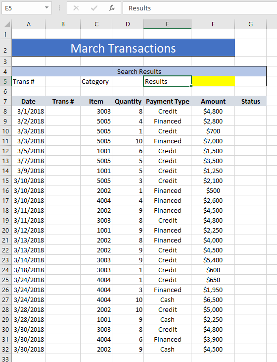
XVfcResults E5 March Transactions Search Results 4 Results 5 Trans # Categor Date Trans # Item Quantity Payment Type Amount status $4,800 $2,800 8 3/1/2018 93/2/2018 10 3/3/2018 11 3/3/2018 12 3/5/2018 13 3/7/2018 14 3/9/2018 15 3/10/2018 16 3/10/2018 17 3/10/2018 18 3/11/2018 19 3/11/2018 20 3/12/2018 21 3/13/2018 22 3/13/2018 23 3/14/2018 24 3/18/2018 25 3/24/2018 26 3/24/2018 27 3/24/2018 28 3/28/2018 29 3/28/2018 30 3/30/2018 31 3/30/2018 32 3/30/2018 3003 Credit 4Financed 1 Credit 10 Financed $7,000 $1,500 $3,500 $1,250 $2,100 Credit 1001 5 Credit 5 Credit 3 Credit 1 Financed 4Financed 9 Financed 1001 2002 $2,600 $4,500 $4,800 $2,250 $4,000 $4,500 2002 3003 1001 2002 2002 3003 3003 Credit 9 Financed 8 Financed Credit Credit 9 1 Credit 1 Credit 3 Financed $1,950 $6,500 $5,000 $2,250 $4,800 $3,900 $4,500 10 10 Cash Credit Cash Credit 2002 1001 3003 6 Financed Cash 2002
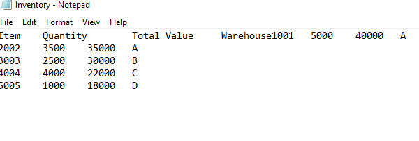
Inventory – Notepad File Edit Format View Help Item Quantity 002 3500 35000 A 003 2500 30000B 0044000 22000 C 5005 1000 18000 D Total Value Warehouse1001 5000 40000 A
Expert Answer
Answer to Grader- Instructions Excel 2016 Project EX16 XL COMP GRADER CAP AS – Manufacturing 1.5 Project Description: You have rec…
OR